Inverse Kinematics is a way to calculate the position that each robot arm joint would need to have in order for the gripper at the end of the arm, called the end-effector, to reach a specific point in space, sometimes with a specific orientation toward that point.

A software plugin that can compute joint positions given the desired goal pose is called an Inverse Kinematics Solver or IK solver.

Open-source IK solvers like KDL and IKFast are easy to setup but only address common scenarios encountered in robotics research labs. If you are building a custom robot, you could look for ways to appease the automated tools until they generate something that works, or learn how to write an IK solver yourself.

Learning about inverse kinematics is another hurdle, as many resources on the subject require extensive mathematical background and fail to provide practical examples, making this subject more complicated than necessary.

This article aims to put you on the fastest path to writing your own solver.

If you’re looking for more background, Introduction to Robotics by Saeed Niku explains inverse kinematics using high-school level math:

The following sections will define important concepts and dive right into working inverse kinematics code examples after a brief survey of approaches.

We will be using MathWorks Matlab or GNU Octave for testing equations and Blender for visualizing solutions and robot geometry.

Both forward and inverse kinematics require describing robot joints. This is often provided in the form of the Universal Robot Description Format (URDF).

The types of joints you’ll be dealing with most often are Revolute and Prismatic. Revolute joints rotate around the joint axis, and prismatic joints slide on it.

In the following video we will use Blender to re-create descriptions for KUKA KR-5 industrial robot, Basic robot arm, and Str1ker drumming robot arm.

Using Blender simplifies working with robot description:

• Each <joint> element in URDF (robot description file) defines a joint.
• The joint <parent> element defines its parent (we will use Make Parent without Inverse to represent this in Blender).
• The joint <origin> element defines the offsets from the previous joint with xyz attribute (translation on X, Y and Z axis in meters) and twists with rpy attribute (roll, pitch, yaw angles in radians).
• The <axis> element defines the axis of rotation or sliding motion.
• The <limit> element defines joint position, velocity, and effort limits.
• The <child> element refers to the child <link> in the same file, which is a 3D model of a segment of the robot arm between the current and the next joint (for example, forearm is between elbow and wrist).
• The corresponding <link> element for the child link contains a <visual> element that usually specifies the <mesh> element with the filename of the 3D model used to represent the link visually.

Once the models for the links associated with each joint are imported in Blender, parent-child relationships are setup, and offsets are specified for each joint, we will be able to use the Blender to calculate forward kinematics and visualize inverse kinematics solutions.

Joints are represented by 4x4 (homogenous) transformation matrices:

• Revolute joints are defined by a revolution around an axis.
• Prismatic joints are defined by a translation on an axis.

Linear and angular offsets from the previous joint are also included:

• Linear offset is usually the length or height of the previous link, and is defined by a constant translation.
• Angular offset (or twist) is any constant rotation that is not on joint axis.

The position of the joint is called a joint variable because it could represent an angle in radians or an offset in meters. Joints may also have more than one degree of freedom (DOF) with one joint variable assigned to each DOF.

Once the robot is assembled in Blender, it’s easy to extract joint matrices.

1. Turn one of the Blender panes into a Python Console. If you haven’t customized anything previously, the Animation pane on the bottom is a great choice for being turned into a console pane. Click the dropdown menu with the clock icon, and choose Python Console pane type under the Scripting category.

2. Name your joints on the Outliner pane displayed on top right. You should be able to expand each joint to see the children.

3. Execute the following in the Python Console to extract the joint matrix (bpy is the Blender Python API singleton):

   bpy.data.objects["joint_name"].matrix_local

4. To extract the position and orientation of the end-effector in world space coordinates, use the matrix_world property:

   bpy.data.objects["end_effector"].matrix_world

If you followed these steps, you’ve just calculated forward kinematics.

It’s helpful to visualize joint coordinate frames by using an Empty Arrows object in Blender. Click Add > Empty > Arrows and parent this new Empty object to the last joint without inverse.

To build a 4x4 joint matrix in GNU Octave, execute the following directly on the command prompt, or save in a .m script and then execute the script:

Once you have the matrices for each of the joints, calculate forward kinematics by multiplying them together to get the end-effector pose:

You may find it easier to use Matlab on the command line much like Octave:

Unlike Octave, Matlab will launch with its system folder as the current directory, so you may have to change the current directory using cd after launching.

To build a 4x4 joint matrix in MathWorks Matlab:

Multiply the joint matrices together to calculate forward kinematics:

Matlab and Octave are essentially Python REPLs. The ... (ellipsis) is used to wrap your code to the next line and % is a single-line comment.

Placing ; at the end of the line will execute the line without echoing the output. Omitting ; will echo the output of the calculation.

The Denavit-Hartenberg (DH) parameters are simply a convention for describing a joint transformation matrix as a function of four parameters:

• Joint offset d: translation on Z axis
• Joint angle θ: rotation on Z axis
• Link length a: translation on X axis
• Joint twist α: rotation on X axis

The Denavit-Hartenberg matrix can be built directly by using the following expressions in each matrix cell, or by multiplying the above transforms:

See Octave and Matlab examples of defining joints using DH parameters and multiplying them together to calculate forward kinematics.

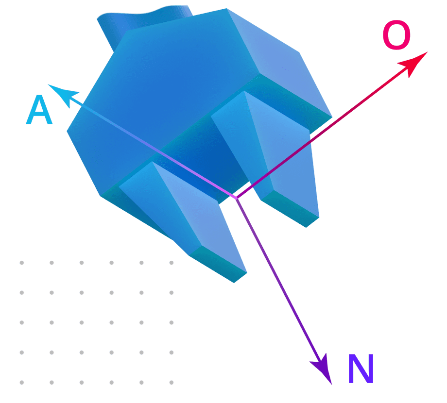
The 4x4 matrix that describes the end-effector pose consists of four vectors:

• The N or Normal unit vector with components nx, ny, nz describes the normal pointing out of the end-effector. Rotation around this vector corresponds to roll in terms of Euler (roll-pitch-yaw) angles.
• The O or Orientation unit vector with components ox, oy, oz is the local up direction, thus rotation around this axis is equivalent to yaw.
• The A or Approach unit vector with components ax, ay, az is the local right direction, thus rotation around this axis is equivalent to pitch.
• The P or Position vector with components px, py, pz describes the position of the end-effector on X, Y, Z axis in world space.

To visualize any of these unit vectors by using the Blender Math Vis Console:

There are several ways to solve inverse kinematics problems:

• Numerical solvers measure changes to end-effector pose resulting from changes in joint variables, until they find a solution within tolerance.
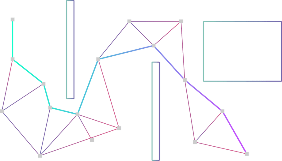
• Sampling-based solvers build a graph of random possible joint states and look for connections that lead to end-effector reaching goal pose.
• Analytical solvers equate the product of all joint matrices with the end-effector pose, and solve the resulting system of nonlinear equations.
• Geometric solvers use trigonometry to break the problem into multiple steps and solve for each joint variable on its own plane.

Numerical solvers iteratively sample poses calculated from combinations of joint variables by using forward kinematics.

Each joint variable is increased or decreased based on whether a change in this variable resulted in the end-effector pose getting closer to or further away from the goal. The search stops when the pose is within tolerance of the goal.

We will look at how to implement gradient descent and newton-raphson iterator numerical solvers in the following two sections.

The amount by which to change each joint variable at each iteration is calculated by using a gradient equation:

1. Increment each joint j at each iteration n by Δ:

   joints_{n, j} = joints_{n - 1, j} + Δ

2. Call the forward kinematics function to get the end-effector pose after this joint was incremented by Δ:

   pose_n = forwardKinematics(joints_n)

3. Compute the error by using a gradient equation: the difference in end-effector poses divided by the difference in joint angles:

   error = (pose_n - pose_{n - 1}) / Δ

   This signed value is used as a weight to pull the joint variable in the direction (+/-) that moves the end-effector closer to the goal.

   Dividing by Δ re-maps the error from world space (since this value comes from subtracting end-effector poses) to joint space, where it’s now expressed in joint units and can be used to do steering.

4. Add the error scaled by a damping factor to the joint variable:

   joints_{n, j} = joints_{n - 1, j} + error × damping

   The damping factor is how many joint units to “steer” toward the goal each iteration. A large damping factor may result in over-steering and missing the goal while a small damping factor will make the journey longer than necessary.

The same gradient strategy is used by bacteria to navigate and can be visualized as a rise-over-run descent down a slope to minimize the error:

We can implement this algorithm in C++ using the Eigen3 library for matrix calculations. First define the forward kinematics function that can take a vector of joint variables and return the end-effector pose:

The algorithm starts by initializing the joint variables with an initial guess, which has a biasing influence on the outcome.

See the complete project in the companion repository.

The newton-raphson iterator algorithm is similar to gradient descent. The amount by which to increase or decrease each joint variable at each iteration is computed by using the Jacobian matrix inverse or transpose.

The Jacobian matrix describes how much the end-effector moves and rotates on each axis in response to each joint variable changing. Its inverse or transpose will give you the influences of joint variables on the end-effector.

This matrix will have as many rows as the dimensions being tracked and as many columns as there are joint variables. In this example we are tracking just three dimensions (end-effector X, Y, and Z).

For each joint j at each iteration n:

1. Increment the joint variable by Δ:

   joints_{n, j} = joints_{n - 1, j} + Δ

2. Compute the resulting change to the end-effector pose by using forward kinematics:

   pose_n = forwardKinematics(joints_n)

3. Calculate the difference between the end-effector poses (in world units), divided by Δ (in joint units), to get the weight this joint has on the end-effector pose, recording it in the Jacobian matrix:

   J_j = (pose_n - pose_{n - 1}) / Δ

4. Compute the error (the difference between the end-effector pose with given joint variables, and the goal pose):

   error = goal - pose_n

5. Add the error to the joint variable. The error is scaled by the influence of this joint on the end-effector pose that’s looked up from the transposed Jacobian matrix (this re-maps the error from world-space to joint-space), and scaled again by a damping factor (how much of a correction to make at each iteration in joint units):

   joints_{n, j} = joints_{n - 1, j} + Jtranspose_j × error × damping

See the complete project in the companion repository.

Sampling-based solvers create a graph of randomly sampled states (each state with different joint variables) and look for a path through this graph that reaches the desired goal pose.

Like other numerical solvers, they use an iterative algorithm which takes time and could fail to find a solution. A unique limitation of sampling solvers is that they require at least 6-DOF to make arbitrary points in space reachable.

It’s useful to know the basic theory behind this type of solver, but we won’t gain much by implementing our own since it would be subject to the same limitations as the KDL solver which works with MoveIt out of the box.

Before we dive into analytical IK theory let’s look at IKFast utility that auto-generates a solver based on the robot description and a solution type.

Install IKFast (and the MoveIt IKFast wrapper that simplifies working with this tool) by following IKFast Kinematics Solver tutorial.

An example of a solver plugin auto-generated by IKFast for the Basic robot arm is provided in the companion repository. See the solver implementation.

In this section we will design an analytical solver in Matlab and export it to working C++ code by following these steps:

1. Equate the product of all joint matrices with the end-effector pose.
2. Multiply both sides by inverse of joint matrices to de-couple joint variables in the equations.
3. The resulting matrix equation breaks down into a system of nonlinear equations (one for each matrix cell).
4. This system of equations is then solved for the joint variables.

You may recall solving systems of linear equations in middle school.

Here’s a refresher from Alan Wake 2 where you must solve a system of equations to access a locked container:

We can model this in Matlab or Octave as follows:

Since B1 and B2 are both expressed in terms of B3, we can substitute them into E1 by using subs so that the sum is expressed only in terms of B3:

E1 now looks like this:

Re-arrange E1 in terms of B3 by using isolate:

E1 now looks like this:

We can now solve E2 for B2 after substituting B3:

E2 now looks like this:

Watch the video in the beginning of this section to confirm the protagonist is able to open the container by entering 496 in the code lock.

Matlab and Octave include a symbolic solver, but it can only handle equations of certain complexity. It is able to solve this particular problem with no issue:

This produces the following output:

We could have used solve immediately after defining these equations, but that won’t work with more complex equations we encounter in the next section.

In the following example we solve inverse kinematics for a 3-DOF robot arm. See the .m files for this example in the companion repository.

Examine equations E1 through E12. You can use vpa for readability (for example vpa(E1, 2) would render E1 to 2 digits of precision). Notice that theta1 is the only variable that appears by itself in equations E3 and E7:

Use isolate to re-write the second equation, exposing cos(theta1):

Printing both equations again, we get:

Solving either equation for theta1 results in two solutions because sin and cos return the same value for different angles depending on the quadrant:

Additionally asin and acos only return real numbers for inputs between -1 and 1, thus the solution would only be valid under those conditions.

The 2-argument inverse tangent (atan2) returns a unique solution as long as we can provide both the sine and the cosine of the same joint variable:

Now that we have a solution for theta1, convert it to C++ by using ccode:

Next we need to solve for theta2 and theta3. Reviewing equations E1 through E12, there are no equations where either variable appears by itself. They are always coupled: to solve for one, you need the other.

We can multiply both sides of the IK equation by inverse of a joint matrix containing one of these variables to de-couple them:

In the above example we over-write the IK equation each time just to show the steps. Re-define the system of equations since both sides have changed:

Many of these equations still have theta2 and theta3 locked up.

However, E4 now has cos(theta2) along with cos(theta1) which is known; theta3 no longer appears in that equation. Similarly, E12 now has sin(theta2) exposed, as theta3 has been moved out to the other side.

Substitute cos(theta1) into E4 by using subs:

Re-arrange E4 to isolate cos(theta2), which we then assign to C2:

To complete the puzzle, isolate sin(theta2) in E12, assigning it to S2:

Now we have sin(theta2) and cos(theta2) which lets us use atan2 to solve for theta2 and convert the solution to C++:

The last joint variable theta3 appears in several equations along with theta1 and theta2 which can be substituted. Let’s pick E2 and E10:

Solving for theta3 was more challenging because all equations had both sin(theta3) and cos(theta3) - it was always expressed in terms of itself.

We had to choose two equations, isolate either sin(theta3) or cos(theta3) in one of the equations, and substitute into the other equation.

With the substitution done, we could proceed with getting atan2 since we had both sin(theta3) and cos(theta3).

In this example we solved analytical inverse kinematics for a 3-DOF robot arm. The companion repository includes another example with 4-DOF robot arm.

This type of inverse kinematics solution uses trigonometry to solve for each joint variable. You will be using a lot of inverse trig functions and identities.

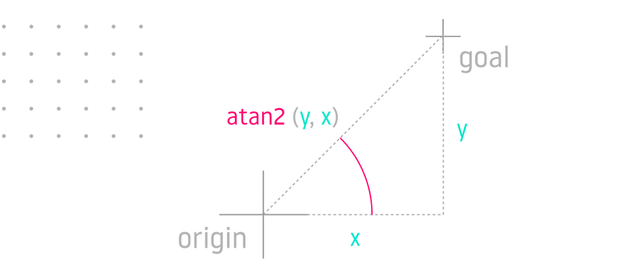
Given cartesian coordinates on a plane, you can solve for the angle with inverse tangent, or arctangent. The 2-argument inverse tangent is preferred because it accounts for the quadrant and therefore returns a unique angle for every input:

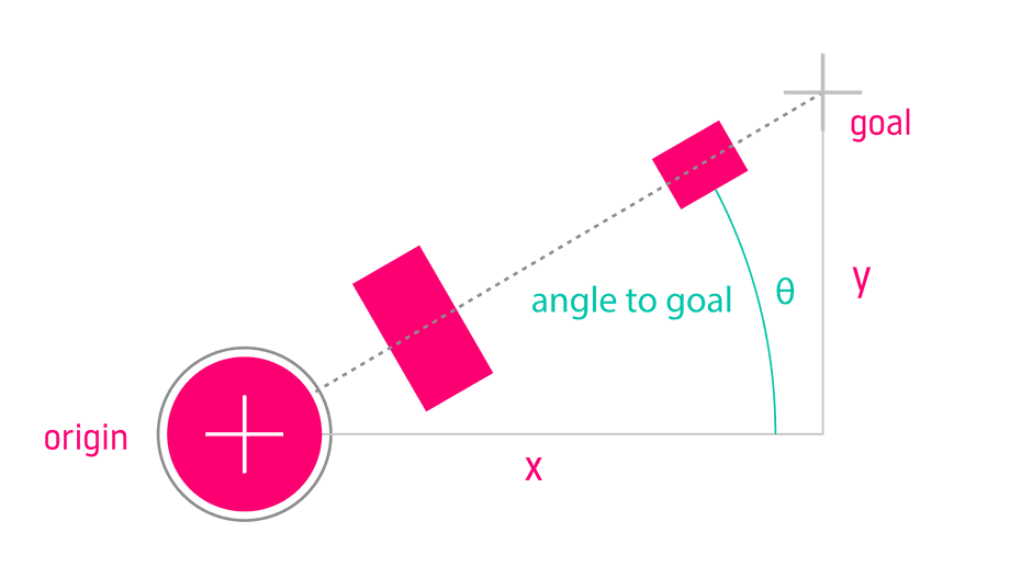
Inverse tangent can be used to solve for the first joint angle θ (theta) of a robot arm mounted on a rotating platform:

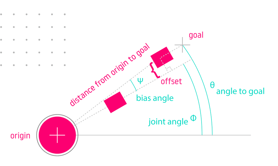
What if the robot arm has joints which are offset from the centerline? This offset would translate into a bias angle added to the basic solution above:

We can describe this problem as a right triangle on XY plane, with its first vertex at the robot origin and second vertex at the goal:

• The hypotenuse is the distance to goal on XY plane.
• The bias angle we need to solve for is Ψ (psi).
• The joint offset is opposite the bias angle.
• We can use inverse sine to solve for this angle because we have the opposite side and the hypotenuse.

Once we have the bias angle Ψ (psi), we can apply it to the angle to goal θ (theta) from the previous section to get the final joint angle Φ (phi):

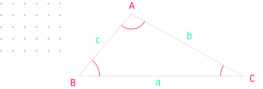
The Law of Cosines can be used when several joints rotate on the same axis. The sides (lower case) are opposite from the angles (upper case):

If you know all three sides you can solve for any of the inner angles:

• cos(A) = (b² + c² - a²) / 2bc
• cos(B) = (a² + c² - b²) / 2ac
• cos(C) = (a² + b² - c²) / 2ab

A pair of links with a common joint can be modeled as a triangle with two sides that are link lengths and the third side that’s a distance from first to last joint:

In the following two examples, we will use the law of cosines to compute the shoulder and elbow angles of a 3-DOF robot arm.

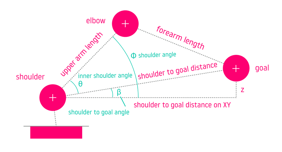
Solve for the inner shoulder angle θ corresponding to angle B in the triangle by isolating it in the equation cos(B) = (a² + c² - b²) / 2ac:

• B: inner shoulder angle
• A: inner elbow angle
• C: inner wrist angle
• c: upper arm link length
• b: forearm link length
• a: the distance between shoulder joint and goal

The inner shoulder angle is not enough to determine the angle of the shoulder joint, since the triangle would be tilted depending on whether the goal is above or below the shoulder joint.

Therefore we need to solve for the shoulder to goal angle β (beta), which describes the angle of that tilt:

This lets us solve for the outer shoulder angle Φ which is the joint angle:

Now we can use the same process to find the elbow joint angle:

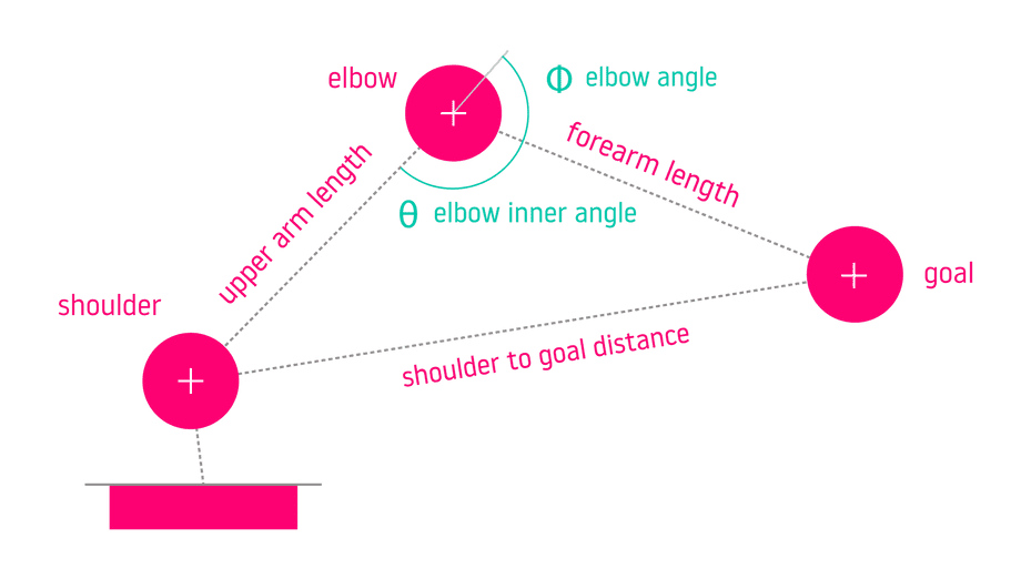
If we label the elbow inner angle as A, then cos(A) = (b² + c² - a²) / 2bc, and to solve for A we take the inverse cosine of the right side:

• B: inner shoulder angle
• A: inner elbow angle
• C: inner wrist angle
• c: upper arm link length
• b: forearm link length
• a: the distance between shoulder joint and goal

The inner elbow angle is a part of the elbow joint angle. For this robot the elbow joint limits are 0 (elbow “straight”) to 180° or π (elbow “closed”).

Subtract the inner elbow angle θ from π to invert the angle in [0 - π] range, then negate the result since the joint variable increases clock-wise, while angles in trigonometric equations are always described counter-clockwise.

In this last example we will compute inverse kinematics for a 4-DOF robot arm, where the angle of the last DOF (the wrist) is fixed or determined externally.

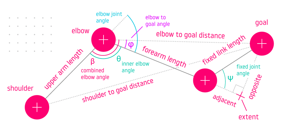
This problem can be represented by three triangles overlaid over each other - one with vertices at shoulder, elbow and goal, another with vertices at wrist, elbow, and goal, and last one with vertices at wrist, goal, and extent:

We need to isolate the inner elbow angle θ between the upper arm and the forearm. This can be done by using the surrounding geometry:

1. Find the unknown sides of the shoulder-elbow-goal triangle: the elbow to goal distance and the shoulder to goal distance.
2. Use the shoulder-elbow-goal triangle to solve for the combined elbow angle β with law of cosines. This angle is a sum of the angle θ we need and the elbow to goal angle φ (phi) which is not yet known.
3. Use the extent-elbow-goal triangle to solve for φ after we find the unknown sides: one opposite the fixed joint angle Ψ (psi) and one a sum of forearm link length and the side adjacent to Ψ.
4. Since β = θ + φ and we know both β and φ, we can solve for θ.
5. Re-map inner elbow angle θ according to joint limits by subtracting from π and negating as in the previous section.

Two of these steps require us to find the sides opposite and adjacent to the fixed joint Ψ (psi). We can use Soh-Cah-Toa trigonometric identities to do this:

Now we can use the larger elbow-goal-extent triangle to find the elbow to goal distance. Because this is a right triangle, its hypotenuse will give you the distance between elbow and goal vertices.

One of the sides in this triangle is opposite the fixed joint. The other is a sum of the forearm link length and the side adjacent to the fixed joint:

The only unknown side of the shoulder-elbow-goal triangle remaining is the shoulder to goal distance on the local XZ plane:

Once all sides of the shoulder-elbow-goal triangle are known, we can use the law of cosines to solve for the combined elbow angle β (beta).

If we take β to be angle A in the law of cosines triangle, then:

cos(A) = (b² + c² - a²) / 2bc

• A: combined elbow angle
• c: upper arm link length
• b: elbow to goal distance
• a: shoulder to goal distance

The last piece needed to isolate θ is the elbow to goal angle φ (phi).

We can use the elbow-goal-extent triangle to solve for φ because it is a right triangle with known sides:

To isolate the inner elbow angle θ, subtract the elbow to goal angle φ from the combined elbow angle β since β is a sum of θ and φ: