Kalman Filtercopy link
Learn about this widely used signal processing algorithm capable of overcoming measurement noise in real time.
overviewcopy link
Kalman filter is a “smart” signal processing algorithm that takes advantage of the way the Universe works and even predicts the future to overcome measurement noise and deliver timely, accurate readings.
This algorithm is ubiquitous: it’s used in autonomous navigation systems like Robot Localization in ROS, for Object Tracking in OpenCV, and inside actuators like Dynamixel where measurements from the absolute encoder are fused with measurements from the quadrature encoder to enable precise positioning.
This filter was first used in the Apollo space program and various defense projects in the early 1960s. It was introduced by Rudolf E. Kálmán in 1960 in his seminal paper, A New Approach to Linear Filtering and Prediction Problems, published in the Journal of Basic Engineering.
backgroundcopy link
In this article I introduce the Kalman Filter in the shortest way possible with practical examples. When you’re ready to go deeper check out Kalman Filter from the Ground Up by Alex Becker at kalmanfilter.net:
why not average?copy link
A basic moving average filter can be implemented as follows:
function output = movingAverageFilter(input, bufferSize)  buffer = ones(bufferSize, 1) * input(1);  output = zeros(length(input), 1);
  for sampleIndex = 1:length(input)    bufferIndex = mod(sampleIndex - 1, bufferSize) + 1;    buffer(bufferIndex) = input(sampleIndex);
    % Output is average of last bufferSize inputs    output(sampleIndex) = ...      sum(buffer) / bufferSize;  endend
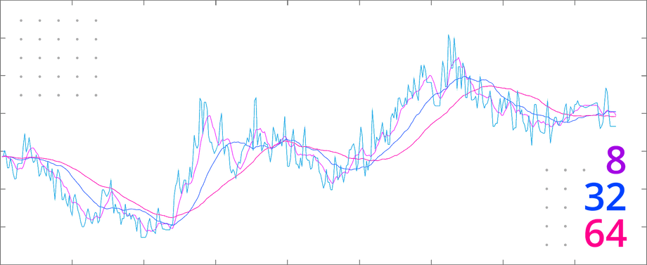
Compare the filter result to the original data with buffer size 8, 32, and 64:
Filtered data has been shifted forward on the time axis proportionately to the smoothing amount, introducing delay:
- In the case of DC motor control for robotics, a moving average filter would cause the PID algorithm to oscillate, as it would see this delay as a signal that it’s not working hard enough, and over-compensate.
- In the case of a vehicle, a moving average would cause the estimated position to lag too far behind, causing the navigation system to suggest changes to the route too late for the driver to respond.
why not low pass?copy link
A basic low-pass filter can be implemented as follows:
function output = lowPassFilter(input, coefficient)  estimate = input(1);  output = zeros(length(input), 1);
  for sampleIndex = 1:length(input)    sample = input(sampleIndex);
    % Output is input blended with previous estimate    estimate = ...      (1.0 - coefficient) * estimate + ...      coefficient * sample;
    output(sampleIndex) = estimate;  endend
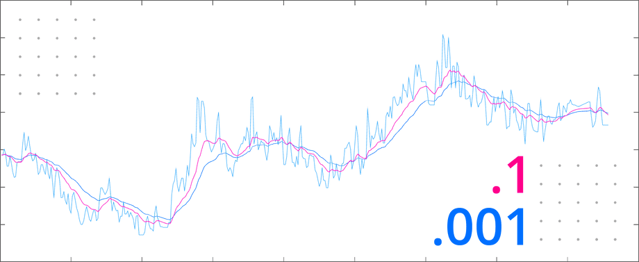
Compare the filter result with 0.1 and 0.001 coefficients to the original data:
This filter missed short temporal spikes in the data. This may be fine if the system is cyclical in nature, but if the subsequent state depends on previous system state, missing events could cause it to diverge far from reality.
In the following video we test both filters on real data:
why predict?copy link
If you know what a moving vehicle or a motor shaft are supposed to do (since you are controlling them in the first place), why should you let measurements have so much influence on where they are estimated to be next?
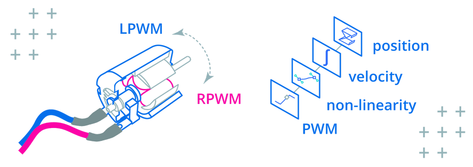
In the case of a DC motor, commanded velocity can be used to determine the current shaft position:
% System Identification (5202 Series Yellow Jacket Motor)MAX_PWM = 65536;MAX_VELOCITY_RPM = 30;MAX_VELOCITY = MAX_VELOCITY_RPM * PI * 2 / 60;PWM_NONLINEARITY = [1.0, 1.023, 1.03, 1.0, 0.98, 1.0];
% System Modelfunction position = systemModel(...  input, ...  position, ...  timeStep ...)  % Map PWM to velocity  norm = input / MAX_PWM;
  index = round(...    length(PWM_NONLINEARITY) * norm...  );
  velocity = ...    norm * PWM_NONLINEARITY[index] * MAX_VELOCITY;
  % Predict position  position = position + velocity * timeStep;end
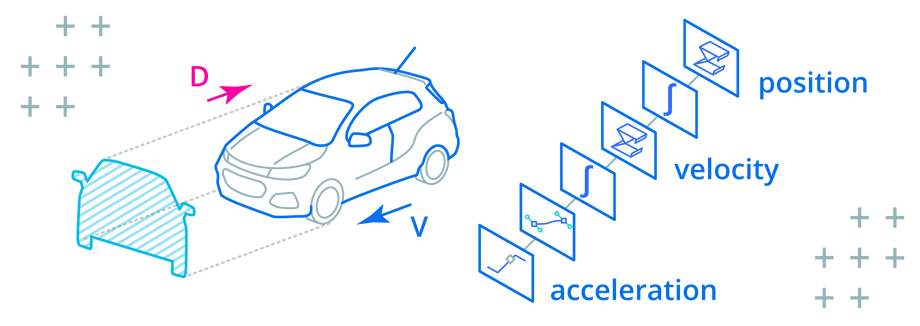
In the case of a moving vehicle, the pressure on the accelerator pedal can determine the velocity and position:
% System Identification (Chevrolet Trax 2017 4WD)MAX_ACCELERATION = 2.82;DRAG_COEFFICIENT = 0.35;FRONTAL_AREA = 2.5;AIR_DENSITY = 1.225;
% System Modelfunction [position, velocity] = systemModel(...  input, ...  position, ...  velocity, ...  timeStep ...)  % Input pressure on accelerator pedal  acceleration = ...    input * MAX_ACCELERATION
  % Subtract drag force  drag = ...    DRAG_COEFFICIENT / 2.0 * ...    AIR_DENSITY * ...    FRONTAL_AREA * ...    velocity^2;
  acceleration = acceleration - drag;
  % Predict position  position = position + velocity * timeStep;
  % Predict velocity  velocity = velocity + acceleration * timeStep;end
Prediction can be a valuable tool provided the model is detailed enough. The Kalman filter’s key strength lies in its ability to combine measurements with predictions, depending on which offers the most accurate estimate.
A basic Kalman filter algorithm looks something like this:
- Start with an initial estimate
- Take a measurement
- Correct the estimate by the measurement
- Predict the next estimate
We will add more detail to these steps in the filter algorithm section later.
variancecopy link
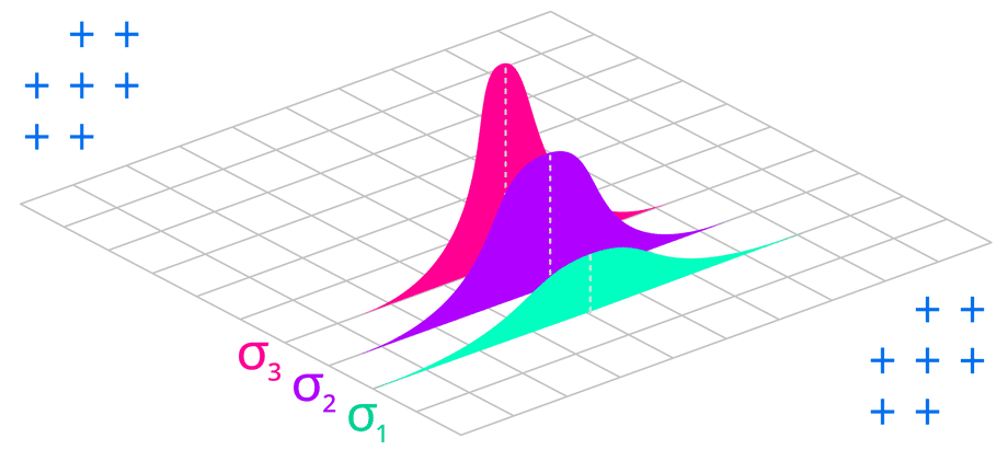
Another special thing about the Kalman filter is that its output isn’t simply a value but a likelihood of it being a certain value. This concept is borrowed from statistics where it’s called a random variable.
- A random variable is defined by a mean and a spread from that mean.
- The mean is a sum of a set of samples divided by the size of the set. This represents the center of the random variable.
- The spread from the mean is called variance and it’s denoted by the greek letter σ (sigma).
- The shape of this spread is a “bell curve” called a Gaussian distribution.
Measuring physical quantities results in readings that follow this Gaussian distribution due to the Holographic Principle of the Universe:
/**/ The one-dimensional array of data that makes up the Universe is stretched over a 3D surface with 1 bit of information every 0.724 x 10-64cm2.
When the Universe is “sampled” by taking a measurement, the sample is interpolated by using a strategy discovered by Carl Gauss: surrounding bits are blended in depending on distance of the sample from the “center” of each bit.
Variance can be calculated from a set of samples as follows:
- Calculate the mean
- For each number in the set, calculate distance from the mean (subtract mean from the number)
- Square each distance from the mean, which will give you variance for this item in the set
- Calculate the mean of all variances in the set (variances summed over number of items). This will give you the variance of the set.
In Matlab or Octave, mean and variance can be calculated as follows:
set = [1, 2, 3, 4, 5]
>> mean(set)
ans =
   3
>> var(set)
ans =
   2.5000
The following video demonstrates how to calculate variance:
filter algorithmcopy link
Since the filter estimate is a random variable, the algorithm has to keep track of its uncertainty, making the same changes to the estimate uncertainty as the ones made to the estimate mean value.
The measurement is also a random variable and its uncertainty could change each iteration or remain constant.
If we include the additional steps for tracking estimate and measurement uncertainties, the algorithm would look like the following:
- Start with initial estimate and its uncertainty
- Take a measurement and determine its uncertainty
- Correct the estimate by the measurement
- Correct the estimate uncertainty by the measurement uncertainty
- Predict the next estimate
- Predict the next estimate uncertainty
Kalman filter starts with an initial estimate, the uncertainty of this estimate, and an initial state of the system being measured.
Each iteration, the system state is corrected by the last measurement according to the ratio of estimate uncertainty to measurement uncertainty.
The next estimate is then predicted by evaluating the system model with the corrected state:
% Initial estimateestimate = y0;
% Initial estimate uncertaintycovariance = P0;
% Initial statestate = x0;
% Identity matrix (state x state)I = eye(length(state));
% Filterfor i = 1:length(inputs)  % Measure  measurement = measurements(i);
  % Determine correction amount  gain = ...    (covariance * C') / ...    (C * covariance * C' + measurementVariance);
  % Correct state with measurement  state = state + gain * (measurement - estimate);
  % Correct estimate uncertainty  covariance = ...    (I - gain * C) * ...    covariance * (I - gain * C)' + ...    gain * measurementVariance * gain';
  % Read input  input = inputs(i);
  % Update state  state = A * state + B * input;
  % Update estimate uncertainty  covariance = A * covariance * A' + noiseCovariance;
  % Predict the next estimate  estimate = C * state + D * input;end
The next few sections will explain the algorithm parameters in more detail.
initial estimatecopy link
The initial estimate y0 can come from initial measurement, output of the system model with initial state, or an educated guess.
A more accurate guess will let the algorithm converge on the optimal estimate faster and avoid a “jump” when the filter performs a large correction.
measurementcopy link
Each iteration begins by taking a measurement (labeled z in equations) and determining its uncertainty or variance, typically denoted by R.
Measurement variance can be constant or vary based on conditions:
- Hall effect encoders like AKSIM report the distance of the rotating magnet from the center of the sensor because this affects the accuracy of the readings. This could be used to derive a measurement variance.
- Complex measurement devices like radar let you estimate the dynamic effects of wind and rain on their signal-to-noise ratio to derive a measurement variance.
- A basic potentiometer can be sampled in a range of expected conditions to calculate a constant variance (see variance).
kalman gaincopy link
To produce optimal estimates, the Kalman filter has to know if the estimates are more or less reliable than measurements.
The ratio of estimate uncertainty to measurement uncertainty is calculated at each iteration. This ratio is called the Kalman gain (typically denoted by K) and used as a weight to correct predictions with measurements.
% K - Kalman gain% P - estimate uncertainty% C - measurement matrix% R - measurement uncertainty
K = (P * C') / (C * P * C' + R);
Similar to other iterative optimization algorithms like Gradient Descent, the Kalman filter has to calculate an error at each iteration, defined as the difference between the prediction and the measurement.
This error is then used to correct the model, with the correction amount determined by the Kalman gain:
- If the measurements are trusted more, the Kalman gain will be closer to
1which will correct the model prediction by a greater amount. - If the model is trusted more, the Kalman gain will be closer to
0which will correct the model prediction by a lesser amount.
Since estimates are a function of the model internal state, we can’t correct them directly. Instead we change the model state to get the desired output:
% Correct state with measurement% x - system state% K - Kalman gain% z - measurement% y - current estimate
x = x + K * (z - y);
After correcting the model state, the estimate uncertainty is updated by blending measurement uncertainty with model uncertainty:
% Correct estimate uncertainty% P - current estimate uncertainty% I - identity matrix (state x state)% K - Kalman gain% C - measurement matrix% R - measurement uncertainty
P = ...  (I - K * C) * ...  P * (I - K * C)' + ...  K * R * K';
If the estimate was based more on the measurement, then the estimate uncertainty reflects more of the measurement uncertainty.
Conversely, if the estimate was based more on the model prediction, then the estimate uncertainty reflects more of the model uncertainty.
predictioncopy link
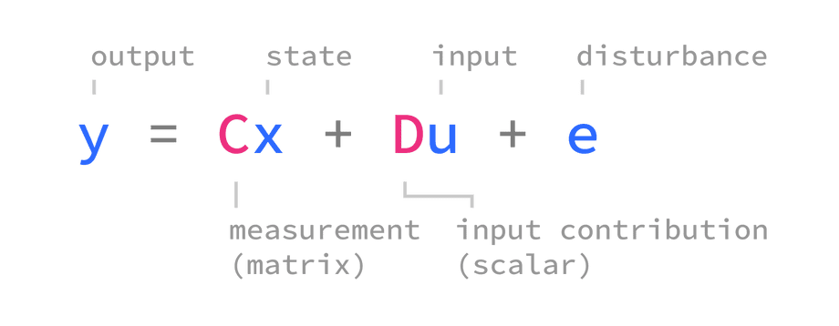
The Kalman filter borrows from System Identification theory which states that most systems (heaters, motors, hydraulic pumps, you name it!) can be approximated by a linear model of the following form:
The system output y depends on system state x and input u.
The relationship between system output and system state is described by C measurement matrix and the relationship between input and immediate output is described by D input contribution.
Differences between the real system and its model are represented by e as disturbance or noise. This is a theoretical term that’s there in the equation to represent “unknowns” and does not appear in the code.
/**/ The measurement matrix is often called
Hin literature, but in this article I useCfor consistency with Matlab System Identification Toolbox.
When modeling systems, you’ll find that the input contribution to system output D is almost always 0 because real-world systems are not instantly affected by inputs. Instead, the inputs modify system state which eventually changes the output.
state transitioncopy link
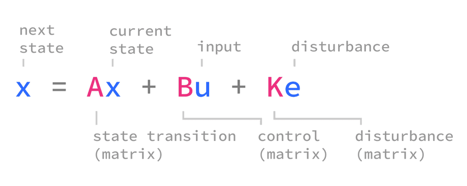
The following equation is used to update (or transition) the state of a linear system model at each iteration:
This equation involves the following terms:
xis the system state being updated. The new state is based on the previous state so this term appears on both sides of the equation. The initial system state is usually denoted byx0.uis the input provided at this iteration.Ais the state transition matrix. Multiplying the system state by this matrix will “simulate” the system, advancing it forward by one time step.Bis the input matrix or control matrix that represents the weight of input on each system state variable. Multiplying the input by this matrix will change each system state variable by a different amount depending on how it’s affected by the input.erepresents the noise or disturbance that affects the system state transition. This is a theoretical term used to model unknowns so it does not appear in the code.Krepresents the influence of noise on each state variable. Sinceeis not used in a practical implementation, we don’t use this term either.
covariancecopy link
For a system model with a single state variable, the initial estimate and disturbance uncertainties are represented by scalar variances.
For a system with multiple state variables, the initial estimate and disturbance uncertainties are represented by square covariance matrices with the same number of rows and columns as there are state variables.
In a covariance matrix, the diagonal entries encode variances, and the off-diagonal entries encode covariances.
estimate covariancecopy link
Estimate uncertainty is typically denoted by P, and the uncertainty of initial estimate is denoted by P0.
For systems with only one state variable both terms are scalar variances, otherwise they are covariance matrices.
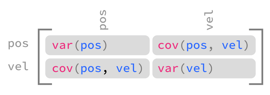
A covariance matrix that encodes the estimate uncertainty of a system with two state variables (position and velocity) would look like this:
This matrix encodes the following information:
- The variance of position (how far the estimated position could be from the true position, squared)
- The variance of velocity (how far the estimated velocity could be from the true velocity, squared)
- The covariance of position and velocity (the mathematical relationship between position and velocity random variables), with
0indicating the two variables are not related.
A covariance matrix that encodes the estimate uncertainty of a system with three or more state variables follows the same pattern:
There are a few ways to initialize the estimate uncertainty:
If the approximate variances of state variables are known, they can be projected on the diagonal of the covariance matrix:
covariance = diag([ ...100, ...200, ...300 ...]);covariance =100 0 00 200 00 0 300If the system was identified with Control System Toolbox, the standard deviations of state variables are available in dx0 property. Squaring elements of
dx0to convert standard deviation to variance and projecting them on the diagonal will give you the estimate covariance:% ss - identified systemcovariance = diag(ss.dx0.^2);5.5288e+13 0 00 1.5450e+19 00 0 2.6517e+21If you have a data set that records system state over time you could use Matlab’s cov function to initialize the estimate covariance:
% CSV with position, velocity, accelerationdataset = readmatrix("states.csv");covariance = cov(dataset);If you can express the variance of the system model in terms of tolerance by using it in a sentence like “this estimate is within x or +/- x”, then square half the tolerance amount to convert it to variance.
The model variance can then be back-projected through the measurement matrix to determine the variance of the initial estimate:
modelTolerance = 50modelVariance = (modelTolerance / 2)^2;covariance = diag( ...inv(C) * ...eye(length(state)) * modelVariance ...* inv(C)' ...);Multiplying variance by another quantity requires squaring that quantity. To make this work with matrices, the variance is pre-multiplied by the matrix and post-multiplied by the transpose of the same matrix. This is why you’ll often see the pattern
X * y * X'.Lastly, you could assume the same variance for all initial state variables, leaving covariances blank:
variance = 200;covariance = eye(length(state)) * variancecovariance =200 0 00 200 00 0 200
These initialization strategies work because the Kalman filter will eventually converge on a more accurate estimate covariance.
However, significantly over-estimating initial estimate uncertainty will cause the algorithm to ignore model predictions while significantly over-estimating the measurement variance will cause the algorithm to ignore measurements.
/**/ Recall that Kalman filter works by calculating a ratio between the two uncertainties, so if either one is many orders of magnitude greater than the other, it will break the filter.
noise covariancecopy link
A process noise or disturbance covariance matrix usually denoted by Q looks exactly like estimate covariance, but it encodes the variance of Gaussian noise affecting the change made to each state variable within a single iteration.
/**/ Noise or disturbance is the difference between the system model and the real system. Its covariance represents the likelihood of state variables being affected by random occurrences like external forces, noise, or the system state being updated using imperfect (noisy) inputs.
There are a few ways to initialize the Q covariance matrix:
Similarly to estimate covariance, the approximate variance of noise or disturbance affecting all state variables in the same way could be projected by spreading the same variance across the diagonal:
noiseVariance = 200noiseCovariance = eye(length(state)) * noiseVarianceIf the approximate variance of noise introduced by updating the system state is known, it could be projected by using the state transition matrix:
noiseVariance = 200;noiseCovariance = A * noiseVariance * A'For systems identified with System Identification Toolbox, the noise variance is available in
NoiseVarianceproperty of the model:% ss1 - linear system modelnoiseCovariance = eye(length(state)) * ss1.NoiseVarianceIf the approximate variance of noise introduced by the system input is known, it could be projected by using the control matrix:
inputNoiseVariance = 200;noiseCovariance = B * inputNoiseVariance * B'If the approximate variances of noise or disturbances affecting each state variable are known, they could be used to fill in diagonal entries of the covariance matrix, leaving off-diagonal entries blank:
noiseCovariance = diag([ ...positionNoiseVariance, ...velocityNoiseVariance, ...accelerationNoiseVariance ...])If the system was identified with Control System Toolbox, the covar function will output its disturbance covariance:
noiseVariance = 200;[ ...% Initial estimate varianceP, ...% Disturbance covarianceQ ...] = covar(ss, noiseVariance)Finally, you could simulate your system model with the same data used to identify it, and calculate the difference between the original measurements and the system model at each iteration.
Since the system model includes a measurement matrix which maps system state to system output, you could multiply the difference between the original measurement and the model prediction by the inverse of this matrix to calculate the noise affecting each state variable at each iteration.
With these results recorded in a separate vector for each state variable, you could then use
covto generate a disturbance matrix.
covariance transitioncopy link
Since Kalman filter estimates are random variables represented by mean and variance, anything that we do to the mean of the estimate must also be reflected in its uncertainty.
Earlier we corrected the estimate uncertainty by the same amount (K) used to correct the estimate:
% P - estimate uncertainty% R - measurement uncertainty% I - identity matrix (state x state)% K - Kalman gain% C - measurement matrix
P = ...  (I - K * C) * P * (I - K * C)' + ...  K * R * K';
In this step, we transition the estimate uncertainty by the same amount (A) used to transition the estimate:
% P - estimate uncertainty% A - state transition matrix% Q - state transition noise/disturbance matrix
P = A * P * A' + Q;
Recall that A is the state transition matrix that represents the change made to the system state at each iteration.
The noise covariance matrix Q represents how much uncertainty is added at each iteration by simulating the system based on an imperfect model and using noisy inputs to change the system state.
system identificationcopy link
The system model can be derived by analyzing the system (as we did in the overly simplified examples of a vehicle and PWM-controlled motor in why predict? section earlier), or by using system identification.
/**/ A system identification algorithm tries to guess the system model given system input and output tracked over time.
In the following video we’ll identify a system in Matlab Control System Toolbox using a discrete linear state-space model:
Identifying a system refers to finding A, B, C, D coefficients that make the output of the linear model most closely resemble the original measurements. These coefficients can then be used as parameters to the Kalman filter.
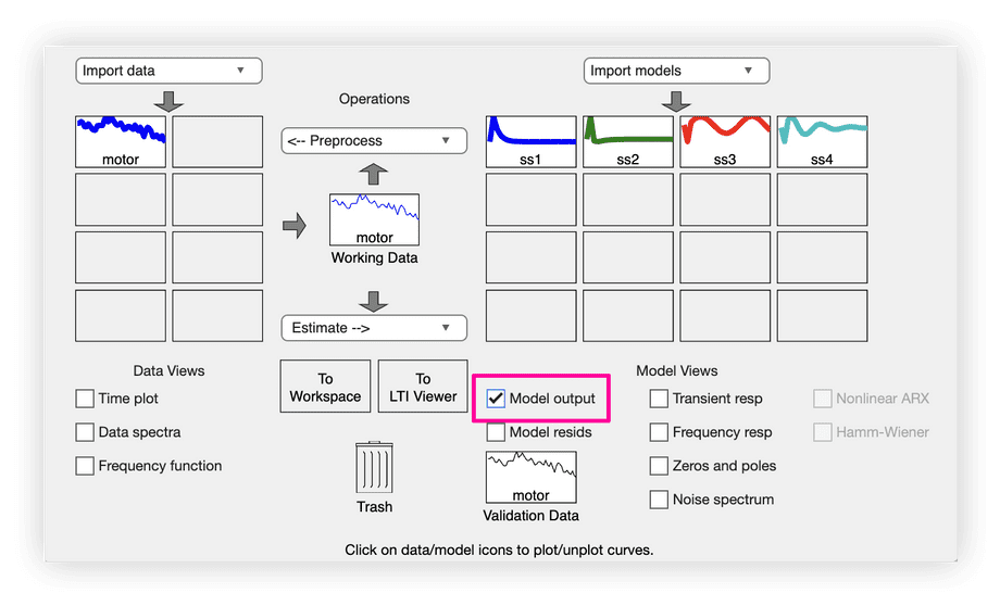
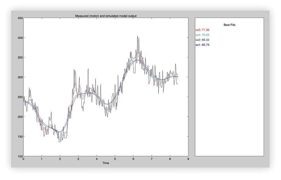
The best way to compare the identified systems to original measurements is by viewing the Model Output in System Identification app:
This will simulate any identified models and display their outputs alongside the original measurements:
The properties of a system identified by Control System Toolbox can be extracted by using an object property notation, for example:
% Get initial state of system "ss1"ss1.x0We will use the following properties in this article:
A,B,C,Dare the coefficients described earlier.x0is the initial system state.dx0is the uncertainty of initial state.NoiseVarianceis the variance of Gaussian noise affecting the system.
For more background on system identification, try this series of tutorials assembled by two professors at Carnegie Mellon university.
simulating systemscopy link
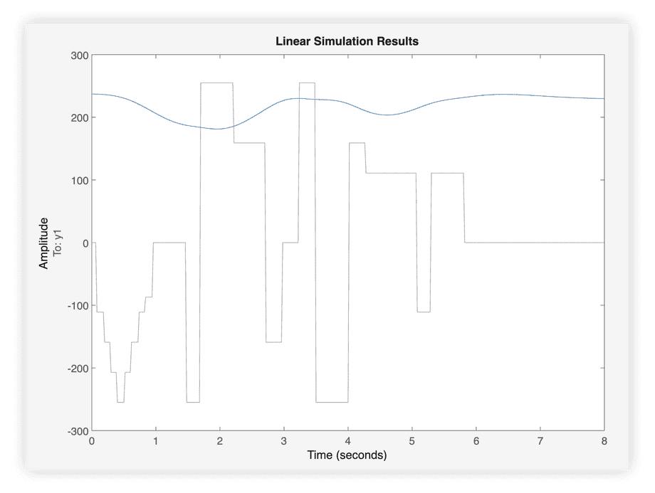
The quickest way to simulate a linear system is by using lsim in Matlab:
% Linear discrete system ssstartTime = 0;endTime = 8;timeStep = ss.Ts;initialState = ss.x0;
% Generate equally spaced time samplestime = startTime:timeStep:endTime;
% Simulatelsim(ss, inputs, time, initialState);
Calling lsim without storing results in a variable will display a plot while assigning to a variable will store the simulated outputs in that variable.
It’s useful to understand how linear system equations presented earlier are used by lsim under the hood to simulate the system.
See the complete Matlab and C++ examples demonstrating how to simulate a linear system in systemid companion repository.
demonstrationcopy link
Live Kalman filter demonstration that lets you load a file and tweak parameters:
| time | reading | PWM |
|---|---|---|
| 0.019995 | 243 | 0 |
| 0.0400168 | 243 | 0 |
| 0.0600218 | 251 | 0 |
| 0.0799967 | 244 | 0 |
| 0.100011 | 228 | -111 |
| 0.120012 | 228 | -111 |
| 0.139993 | 241 | -111 |
| 0.160019 | 232 | -111 |
| 0.180016 | 220 | -111 |
| 0.20001 | 213 | -111 |
| 0.220012 | 214 | -159 |
| 0.240088 | 233 | -159 |
| 0.260076 | 234 | -159 |
| 0.280015 | 234 | -159 |
| 0.300022 | 234 | -159 |
| 0.32002 | 258 | -207 |
| 0.340016 | 273 | -207 |
| 0.360013 | 249 | -207 |
| 0.380027 | 255 | -207 |
| 0.400015 | 268 | -207 |
| 0.420026 | 255 | -255 |
| 0.440058 | 242 | -255 |
| 0.459996 | 235 | -255 |
| 0.480028 | 237 | -255 |
| 0.500021 | 245 | -255 |
| 0.520013 | 233 | -255 |
| 0.540016 | 217 | -207 |
| 0.559992 | 220 | -207 |
| 0.58001 | 230 | -207 |
| 0.60008 | 230 | -207 |
| 0.620022 | 222 | -207 |
| 0.640024 | 217 | -159 |
| 0.659993 | 236 | -159 |
| 0.680031 | 218 | -159 |
| 0.700009 | 211 | -159 |
| 0.720011 | 227 | -159 |
| 0.740012 | 207 | -159 |
| 0.760001 | 186 | -111 |
| 0.779996 | 213 | -111 |
| 0.8 | 226 | -111 |
| 0.820014 | 221 | -111 |
| 0.84001 | 209 | -111 |
| 0.860022 | 186 | -87 |
| 0.880019 | 186 | -87 |
| 0.900019 | 194 | -87 |
| 0.920004 | 182 | -87 |
| 0.940023 | 177 | -87 |
| 0.960017 | 191 | -87 |
| 0.980083 | 171 | 0 |
| 1.00002 | 165 | 0 |
| 1.02001 | 188 | 0 |
| 1.04001 | 193 | 0 |
| 1.06002 | 183 | 0 |
| 1.08001 | 172 | 0 |
| 1.1 | 166 | 0 |
| 1.12001 | 156 | 0 |
| 1.14002 | 150 | 0 |
| 1.16002 | 150 | 0 |
| 1.18001 | 155 | 0 |
| 1.20001 | 166 | 0 |
| 1.22001 | 174 | 0 |
| 1.24002 | 166 | 0 |
| 1.26008 | 157 | 0 |
| 1.28001 | 154 | 0 |
| 1.30001 | 162 | 0 |
| 1.32002 | 169 | 0 |
| 1.34001 | 168 | 0 |
| 1.36 | 155 | 0 |
| 1.38003 | 158 | 0 |
| 1.39999 | 182 | 0 |
| 1.41999 | 199 | 0 |
| 1.43999 | 199 | 0 |
| 1.46003 | 194 | 0 |
| 1.48 | 190 | 0 |
| 1.5 | 193 | -255 |
| 1.52002 | 198 | -255 |
| 1.54002 | 212 | -255 |
| 1.56002 | 189 | -255 |
| 1.58 | 168 | -255 |
| 1.6 | 180 | -255 |
| 1.62001 | 173 | -255 |
| 1.63999 | 168 | -255 |
| 1.66001 | 169 | -255 |
| 1.68001 | 153 | -255 |
| 1.7 | 161 | -255 |
| 1.72001 | 161 | 255 |
| 1.74002 | 180 | 255 |
| 1.76001 | 164 | 255 |
| 1.78002 | 164 | 255 |
| 1.80004 | 168 | 255 |
| 1.81999 | 160 | 255 |
| 1.84002 | 166 | 255 |
| 1.86002 | 162 | 255 |
| 1.88002 | 157 | 255 |
| 1.90001 | 144 | 255 |
| 1.92007 | 161 | 255 |
| 1.94 | 162 | 255 |
| 1.95999 | 136 | 255 |
| 1.97999 | 136 | 255 |
| 2.00001 | 136 | 255 |
| 2.02002 | 136 | 255 |
| 2.04001 | 140 | 255 |
| 2.06001 | 155 | 255 |
| 2.08001 | 161 | 255 |
| 2.10002 | 150 | 255 |
| 2.12002 | 144 | 255 |
| 2.14001 | 144 | 255 |
| 2.16009 | 141 | 255 |
| 2.18001 | 165 | 255 |
| 2.20002 | 175 | 255 |
| 2.22 | 159 | 255 |
| 2.24002 | 154 | 159 |
| 2.26 | 147 | 159 |
| 2.28003 | 147 | 159 |
| 2.3 | 146 | 159 |
| 2.32002 | 146 | 159 |
| 2.34002 | 146 | 159 |
| 2.36001 | 146 | 159 |
| 2.37999 | 153 | 159 |
| 2.40001 | 152 | 159 |
| 2.42002 | 190 | 159 |
| 2.44001 | 204 | 159 |
| 2.46 | 209 | 159 |
| 2.48002 | 225 | 159 |
| 2.5 | 202 | 159 |
| 2.52002 | 194 | 159 |
| 2.54001 | 204 | 159 |
| 2.56001 | 212 | 159 |
| 2.58002 | 212 | 159 |
| 2.60002 | 195 | 159 |
| 2.62 | 207 | 159 |
| 2.64003 | 229 | 159 |
| 2.66 | 215 | 159 |
| 2.68002 | 237 | 159 |
| 2.70002 | 271 | 159 |
| 2.72002 | 258 | 159 |
| 2.74002 | 254 | -159 |
| 2.76 | 259 | -159 |
| 2.78 | 320 | -159 |
| 2.80001 | 316 | -159 |
| 2.82002 | 273 | -159 |
| 2.84 | 315 | -159 |
| 2.86001 | 315 | -159 |
| 2.88002 | 306 | -159 |
| 2.90002 | 270 | -159 |
| 2.92002 | 262 | -159 |
| 2.94001 | 262 | -159 |
| 2.95999 | 253 | -159 |
| 2.98002 | 247 | -159 |
| 3.00002 | 251 | 0 |
| 3.02002 | 256 | 0 |
| 3.04002 | 262 | 0 |
| 3.06002 | 288 | 0 |
| 3.08001 | 300 | 0 |
| 3.09999 | 263 | 0 |
| 3.12001 | 246 | 0 |
| 3.14003 | 258 | 0 |
| 3.15999 | 258 | 0 |
| 3.18001 | 251 | 0 |
| 3.2 | 227 | 0 |
| 3.22 | 221 | 0 |
| 3.24004 | 226 | 0 |
| 3.26 | 222 | 255 |
| 3.28002 | 214 | 255 |
| 3.3 | 230 | 255 |
| 3.32002 | 236 | 255 |
| 3.3401 | 234 | 255 |
| 3.36 | 249 | 255 |
| 3.38 | 253 | 255 |
| 3.40001 | 258 | 255 |
| 3.42 | 258 | 255 |
| 3.44003 | 268 | 255 |
| 3.46002 | 262 | 255 |
| 3.48001 | 280 | 255 |
| 3.50002 | 272 | 255 |
| 3.52002 | 251 | -255 |
| 3.54001 | 317 | -255 |
| 3.56002 | 321 | -255 |
| 3.58 | 258 | -255 |
| 3.60002 | 269 | -255 |
| 3.62002 | 274 | -255 |
| 3.64 | 250 | -255 |
| 3.66 | 256 | -255 |
| 3.68002 | 262 | -255 |
| 3.70002 | 259 | -255 |
| 3.72002 | 259 | -255 |
| 3.74001 | 246 | -255 |
| 3.76 | 236 | -255 |
| 3.78005 | 248 | -255 |
| 3.80001 | 282 | -255 |
| 3.82 | 275 | -255 |
| 3.84002 | 263 | -255 |
| 3.86001 | 273 | -255 |
| 3.88 | 261 | -255 |
| 3.90001 | 266 | -255 |
| 3.92001 | 257 | -255 |
| 3.94003 | 268 | -255 |
| 3.96001 | 296 | -255 |
| 3.98 | 261 | -255 |
| 4 | 230 | -255 |
| 4.02 | 230 | -255 |
| 4.04 | 240 | 159 |
| 4.06001 | 267 | 159 |
| 4.08 | 279 | 159 |
| 4.10002 | 251 | 159 |
| 4.12001 | 233 | 159 |
| 4.14001 | 233 | 159 |
| 4.16 | 227 | 159 |
| 4.18001 | 241 | 159 |
| 4.20002 | 230 | 159 |
| 4.22 | 266 | 159 |
| 4.24002 | 282 | 159 |
| 4.26 | 241 | 159 |
| 4.28002 | 238 | 159 |
| 4.30001 | 238 | 111 |
| 4.32001 | 226 | 111 |
| 4.34002 | 228 | 111 |
| 4.36002 | 243 | 111 |
| 4.38001 | 243 | 111 |
| 4.4 | 241 | 111 |
| 4.42002 | 241 | 111 |
| 4.44001 | 223 | 111 |
| 4.46001 | 219 | 111 |
| 4.48008 | 210 | 111 |
| 4.50001 | 201 | 111 |
| 4.52008 | 207 | 111 |
| 4.54001 | 226 | 111 |
| 4.56002 | 209 | 111 |
| 4.58 | 209 | 111 |
| 4.60007 | 199 | 111 |
| 4.62002 | 199 | 111 |
| 4.64002 | 215 | 111 |
| 4.66002 | 243 | 111 |
| 4.68002 | 232 | 111 |
| 4.70002 | 212 | 111 |
| 4.72001 | 216 | 111 |
| 4.74001 | 231 | 111 |
| 4.76008 | 218 | 111 |
| 4.78002 | 209 | 111 |
| 4.80001 | 220 | 111 |
| 4.82001 | 231 | 111 |
| 4.84001 | 232 | 111 |
| 4.86002 | 252 | 111 |
| 4.88011 | 252 | 111 |
| 4.90001 | 257 | 111 |
| 4.92004 | 260 | 111 |
| 4.94003 | 251 | 111 |
| 4.96001 | 224 | 111 |
| 4.98002 | 233 | 111 |
| 5.00002 | 257 | 111 |
| 5.02003 | 282 | 111 |
| 5.04001 | 270 | 111 |
| 5.06002 | 233 | 111 |
| 5.07999 | 217 | 111 |
| 5.10001 | 237 | -111 |
| 5.12 | 225 | -111 |
| 5.14002 | 238 | -111 |
| 5.16001 | 238 | -111 |
| 5.18002 | 305 | -111 |
| 5.20002 | 281 | -111 |
| 5.22009 | 253 | -111 |
| 5.24002 | 269 | -111 |
| 5.26 | 264 | -111 |
| 5.28 | 267 | -111 |
| 5.3 | 276 | -111 |
| 5.32002 | 288 | 111 |
| 5.34002 | 272 | 111 |
| 5.36002 | 262 | 111 |
| 5.38004 | 278 | 111 |
| 5.40005 | 259 | 111 |
| 5.42002 | 259 | 111 |
| 5.44 | 295 | 111 |
| 5.46001 | 300 | 111 |
| 5.48003 | 294 | 111 |
| 5.50002 | 308 | 111 |
| 5.52002 | 292 | 111 |
| 5.54001 | 320 | 111 |
| 5.56001 | 321 | 111 |
| 5.58 | 313 | 111 |
| 5.60002 | 309 | 111 |
| 5.62002 | 311 | 111 |
| 5.64002 | 321 | 111 |
| 5.66001 | 312 | 111 |
| 5.68001 | 338 | 111 |
| 5.7001 | 329 | 111 |
| 5.72002 | 329 | 111 |
| 5.74001 | 320 | 111 |
| 5.76 | 347 | 111 |
| 5.78003 | 333 | 111 |
| 5.8 | 325 | 111 |
| 5.82001 | 317 | 111 |
| 5.84001 | 348 | 0 |
| 5.86001 | 364 | 0 |
| 5.88001 | 348 | 0 |
| 5.90001 | 364 | 0 |
| 5.92002 | 357 | 0 |
| 5.94002 | 341 | 0 |
| 5.96001 | 341 | 0 |
| 5.98003 | 341 | 0 |
| 6.00002 | 341 | 0 |
| 6.02001 | 328 | 0 |
| 6.04002 | 312 | 0 |
| 6.06001 | 310 | 0 |
| 6.08001 | 310 | 0 |
| 6.10003 | 310 | 0 |
| 6.12 | 310 | 0 |
| 6.14002 | 342 | 0 |
| 6.16003 | 369 | 0 |
| 6.18001 | 360 | 0 |
| 6.20001 | 335 | 0 |
| 6.22 | 336 | 0 |
| 6.24001 | 404 | 0 |
| 6.26 | 397 | 0 |
| 6.28 | 360 | 0 |
| 6.30002 | 360 | 0 |
| 6.32002 | 400 | 0 |
| 6.34003 | 377 | 0 |
| 6.36001 | 333 | 0 |
| 6.38002 | 362 | 0 |
| 6.4 | 362 | 0 |
| 6.42002 | 333 | 0 |
| 6.44002 | 367 | 0 |
| 6.46003 | 361 | 0 |
| 6.48009 | 321 | 0 |
| 6.5 | 321 | 0 |
| 6.51999 | 346 | 0 |
| 6.54001 | 350 | 0 |
| 6.56002 | 318 | 0 |
| 6.58001 | 318 | 0 |
| 6.60002 | 319 | 0 |
| 6.62001 | 323 | 0 |
| 6.64003 | 307 | 0 |
| 6.66001 | 323 | 0 |
| 6.68001 | 349 | 0 |
| 6.70002 | 338 | 0 |
| 6.72002 | 315 | 0 |
| 6.73999 | 307 | 0 |
| 6.76 | 312 | 0 |
| 6.78002 | 313 | 0 |
| 6.80001 | 320 | 0 |
| 6.81999 | 330 | 0 |
| 6.84001 | 313 | 0 |
| 6.86 | 283 | 0 |
| 6.88002 | 283 | 0 |
| 6.90008 | 287 | 0 |
| 6.92003 | 287 | 0 |
| 6.94003 | 306 | 0 |
| 6.95999 | 320 | 0 |
| 6.98002 | 301 | 0 |
| 7.00002 | 314 | 0 |
| 7.02002 | 321 | 0 |
| 7.04002 | 306 | 0 |
| 7.06002 | 314 | 0 |
| 7.08012 | 329 | 0 |
| 7.10004 | 317 | 0 |
| 7.12001 | 300 | 0 |
| 7.14001 | 278 | 0 |
| 7.16009 | 281 | 0 |
| 7.18002 | 281 | 0 |
| 7.20002 | 330 | 0 |
| 7.22001 | 321 | 0 |
| 7.23999 | 299 | 0 |
| 7.26001 | 305 | 0 |
| 7.28002 | 289 | 0 |
| 7.30001 | 285 | 0 |
| 7.32002 | 276 | 0 |
| 7.34 | 278 | 0 |
| 7.36 | 297 | 0 |
| 7.38002 | 281 | 0 |
| 7.4 | 258 | 0 |
| 7.42001 | 292 | 0 |
| 7.44 | 312 | 0 |
| 7.46002 | 312 | 0 |
| 7.48001 | 293 | 0 |
| 7.5 | 282 | 0 |
| 7.52008 | 276 | 0 |
| 7.54001 | 275 | 0 |
| 7.56003 | 274 | 0 |
| 7.58001 | 274 | 0 |
| 7.60002 | 295 | 0 |
| 7.62 | 317 | 0 |
| 7.64002 | 290 | 0 |
| 7.65999 | 261 | 0 |
| 7.68001 | 275 | 0 |
| 7.70002 | 287 | 0 |
| 7.72001 | 295 | 0 |
| 7.74002 | 295 | 0 |
| 7.76 | 286 | 0 |
| 7.78001 | 284 | 0 |
| 7.80002 | 290 | 0 |
| 7.82002 | 290 | 0 |
| 7.84002 | 294 | 0 |
| 7.86 | 307 | 0 |
| 7.88002 | 313 | 0 |
| 7.90001 | 289 | 0 |
| 7.92001 | 292 | 0 |
| 7.94001 | 309 | 0 |
| 7.96001 | 305 | 0 |
| 7.98003 | 300 | 0 |
| 8.00002 | 312 | 0 |
| 8.02002 | 312 | 0 |
| 8.04002 | 317 | 0 |
| 8.06002 | 311 | 0 |
| 8.07999 | 310 | 0 |
| 8.10002 | 310 | 0 |
| 8.12 | 309 | 0 |
| 8.14002 | 308 | 0 |
| 8.1601 | 308 | 0 |
| 8.29271 | 314 | 0 |
| 8.31277 | 314 | 0 |
| 8.33279 | 295 | 0 |
| 8.35281 | 280 | 0 |
| 8.37279 | 283 | 0 |
| 8.3928 | 289 | 0 |
| 8.41279 | 313 | 0 |
| 8.43279 | 334 | 0 |
| 8.4528 | 328 | 0 |
| 8.47278 | 301 | 0 |
| 8.49286 | 283 | 0 |
| 8.51277 | 283 | 0 |
| 8.53289 | 283 | 0 |
| 8.5529 | 283 | 0 |
| 8.57289 | 283 | 0 |
Enter filter parameters:
kalman in matlabcopy link
The kalman companion repository includes a complete filter implementation in addition to two live notebooks that explain the filter algorithm parameters.
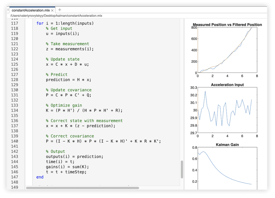
The constantAcceleration.mlx notebook implements a Kalman filter that works with a simpler Newtonian motion model:
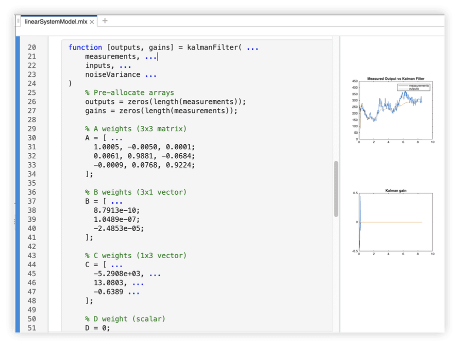
The linearSystemModel.mlx notebook implements a Kalman filter that works with a general-form linear discrete system model:
Finally, kalman.m demonstrates a Kalman filter with the same linear system model in the form of a .m script:
% Constantsglobal A;global B;global C;global D;global Q;global R;global I;
% A weights (3x3 matrix)A = [ ...  1.0005, -0.0050, 0.0001;  0.0061, 0.9881, -0.0684;  -0.0009, 0.0768, 0.9224;];
% B weights (3x1 vector)B = [ ...  8.7913e-10;  1.0489e-07;  -2.4853e-05;];
% C weights (1x3 vector)C = [ ...  -5.2908e+03, ...  13.0803, ...  -0.6389 ...];
% D weight (scalar)D = 0;
% Initial state (3x1 vector)x0 = [ ...  -0.0461;  -0.0198;  0.0098;];
% Initial state standard deviation (3x1 vector)dx0 = [ ...  7.4356e+06;  3.9306e+09;  5.1495e+10;];
% State identity matrixI = eye(length(x0));
% Noise variance (scalar)NoiseVariance = 1.539e-7;
% Noise covariance (3x3 matrix)Q = I * NoiseVariance;
% Measurement varianceR = 3.4556e+03;
% Initial covarianceP0 = diag(dx0.^2);
% Read inputcsv = readmatrix('https://raw.githubusercontent.com/01binary/kalman/main/input.csv');time = csv(:,1);measurements = csv(:,2);inputs = csv(:,3);
% Initializestate = x0;covariance = P0;gain = I * 0;prediction = 100;outputs = zeros(length(inputs), 1);gains = zeros(length(inputs), 1);
% Filterfor i = 1:length(inputs)  % Read input  input = inputs(i);
  % Take measurement  measurement = measurements(i);
  % Correct state  [state, covariance, gain] = kalmanFilter( ...    prediction, ...    measurement, ...    state, ...    covariance, ...    gain ...  );
  % Predict and update state  [state, prediction] = systemModel( ...    state, ...    input ...  );
  % Output  gains(i) = sum(gain);  outputs(i) = prediction;end
function [x, y] = systemModel(x, u)  global A;  global B;  global C;  global D;  global Q;
  % Predict  % y = Cx + Du  y = ...    % Contribution of state    C * x + ...    % Contribution of input    D * u;
  % Update state  % x = Ax + Bu  x = ...    % Contribution of previous state    A * x + ...    % Contribution of input    B * u;end
function [x, P, K] = kalmanFilter(y, z, x, P, K)  global A;  global C;  global Q;  global R;  global I;
  % Update covariance  P = A * P * A' + Q;
  % Optimize gain  K = (P * C') / (C * P * C' + R);
  % Correct state with measurement  x = x + K * (z - y);
  % Correct covariance  P = (I - K * C) * P * (I - K * C)' + ...    K * R * K';end
kalman in c++copy link
The kalman companion repository includes the following example. Steps that can be used to compile, run, and debug the code are in the readme file:
//// Includes//
#include <iostream>#include <fstream>#include <vector>#include <string>#include <random>#include <limits>#include <Eigen/Dense>
//// Namespaces//
using namespace std;using namespace Eigen;
//// Constants//
// A weights (3x3 matrix)const MatrixXd A{  { 0.998800,   0.05193, -0.02261 },  { 0.0222200, -0.01976,  0.7353  },  { 0.0009856, -0.20930, -0.5957  }};
// B weights (3x1 vector)const VectorXd B {{  -0.00000266,  0.0000572747,  -0.0001872152}};
// C weights (1x3 vector)const RowVectorXd C {{  -5316.903919,  24.867656,  105.92416}};
// D weight (scalar)const double D = 0;
// Initial state (3x1 vector)const VectorXd x0 {{  -0.0458,  0.0099,  -0.0139}};
// State standard deviation (3x1 vector)const VectorXd dx0 {{  7.4356e+06,  3.9306e+09,  5.1495e+10}};
// State identity (3x3 matrix)const Matrix3d I = Matrix3d::Identity();
// Noise variance (scalar)const double NoiseVariance = 1.539e-7;
// Noise covariance (3x3 matrix)const MatrixXd Q = I * NoiseVariance;
// Measurement varianceconst double R = 3.4556e+03;
// Initial covarianceconst MatrixXd P0 {{  { pow(dx0(0, 0), 2), 0.0, 0.0 },  { 0.0, pow(dx0(1, 0), 2), 0.0 },  { 0.0, 0.0, pow(dx0(2, 0), 2) }}};
//// Functions//
double systemModel(  VectorXd& x,  // state  double u)     // input{  // Predict  // y = Cx + Du  double y =    // Contribution of state    C.dot(x) +    // Contribution of input    D * u;
  // Update state  // x = Ax + Bu  x =    // Contribution of previous state    A * x +    // Contribution of input    B * u;
  return y;}
double kalmanFilter(  double y,    // prediction  double z,    // measurement  VectorXd& x, // state  MatrixXd& P, // covariance  VectorXd& K) // gain{  // Update covariance  P = A * P * A.transpose() + Q;
  // Optimize gain  K = (    (P * C.transpose()) /    (C * P * C.transpose() + R)  );
  // Correct state with measurement  x = x + K * (z - y);
  // Correct covariance  P = (I - K * C) * P *    (I - K * C).transpose() +    K * R * K.transpose();
  return y;}
//// Forward Declarations//
bool openInput(const string& path, ifstream& file);bool openOutput(const string& path, ofstream& file);bool read(  ifstream& file,  double& time,  double& measurement,  double& input);
//// Entry point//
int main(int argc, char** argv){  ifstream inputFile;
  if (!openInput("input.csv", inputFile))  {    cerr << "Failed to open input file" << endl;    return 1;  }
  ofstream outputFile;
  if (!openOutput("output.csv", outputFile))  {    cerr << "Failed to open output file" << endl;    return 1;  }
  // Initialize  VectorXd state = x0;  VectorXd gain(3);  MatrixXd covariance = P0;  double time, measurement, input;  double prediction = 0.0;
  // Filter  while(read(inputFile, time, measurement, input))  {    // Correct state with measurement    double estimate = kalmanFilter(      prediction,      measurement,      state,      covariance,      gain    );
    // Predict and update state    prediction = systemModel(      state,      input    );
    // Output    outputFile      << time << ","      << estimate << ","      << measurement      << endl;  }
  return 0;}
//// Utilities//
bool openOutput(  const string& path, ofstream& file){  // Delete if exists  remove(path.c_str());
  // Open file for writing  file.open(path);  if (!file.is_open()) return false;
  // Write headers  file << "time,estimate,measurement" << endl;
  return true;}
bool openInput(  const string& path, ifstream& file){  // Open file for reading  file.open(path);  if (!file.is_open()) return false;
  // Skip headers  string headers;  getline(file, headers);
  return true;}
bool read(  ifstream& file,  double& time,  double& measurement,  double& input){  static string line;  getline(file, line);
  sscanf(    line.c_str(),    "%lf, %lf, %lf",    &time,    &measurement,    &input);
return !file.eof();}sensor fusioncopy link
When the same measurement is available from multiple sources, readings can be combined by using a technique called sensor fusion.
/**/ For example, you might have readings from an absolute and a relative encoder, or an odometer and an accelerometer.
The measurements and their uncertainties are combined into a single measurement and its uncertainty with the following equations.
Combined measurement uncertainty
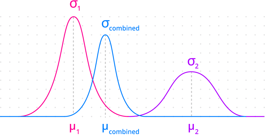
σis the blend of all uncertainties, each weighted by its inverse:σ = 1 / (1 / σ1 + 1 / σn)
Since “one divided by uncertainty” converts it to “certainty” (its opposite), the inner equation sums up all the weighted certainties, and the outer equation converts the result back to “uncertainty”.
Combined measurement mean
μis the blend of all measurements, each weighted by inverse of its uncertainty:μ = σ × (μ1 / σ1 + μn / σn)
This results in the combined measurement that blends in more certain measurement sources in greater amounts.
Combining more measurements results in the combined measurement uncertainty less than the uncertainty of any one measurement:
These equations are simple to implement as two loops that accumulate values:
% Same measurement from multiple sourcesmeasurements = [ 100, 120, 89 ];
% Each source may have a different uncertaintymeasurementVariances = [ 1000, 800, 90000 ];
% Combine measurement uncertaintiessumVariances = 0;
for n = 1:length(measurementVariances)  % Each uncertainty weighted by its inverse  sumVariances = sumVariances + ...    1 / measurementVariances(n);end
measurementVariance = 1 / sumVariances
% Combine measurementssumMeasurements = 0;
for n = 1:length(measurements)  % Each measurement weighted by inverse of its uncertainty  sumMeasurements = sumMeasurements + ...    measurements(n) / measurementVariances(n);end
measurement = sumMeasurements * measurementVariance

>> measurementVariance =
  442.2604
>> measurement =
  111.0025
The resulting measurement (z) and its variance (R) are simply plugged into the Kalman filter, with no changes required to the filter implementation.
For sensor fusion in systems with multiple outputs and other advanced scenarios, see the Kalman Filter from the Ground Up book.
rate mismatchcopy link
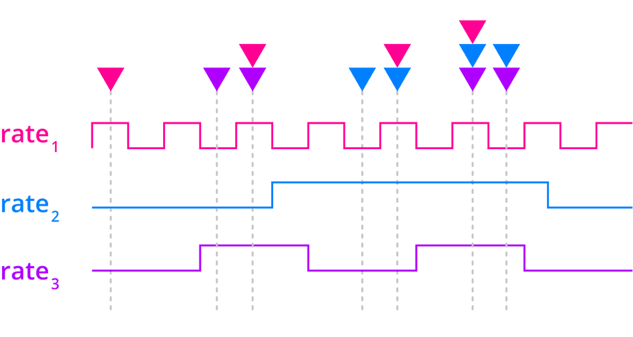
To fuse measurements taken at different rates, simply combine any measurements available during a single Kalman filter iteration:
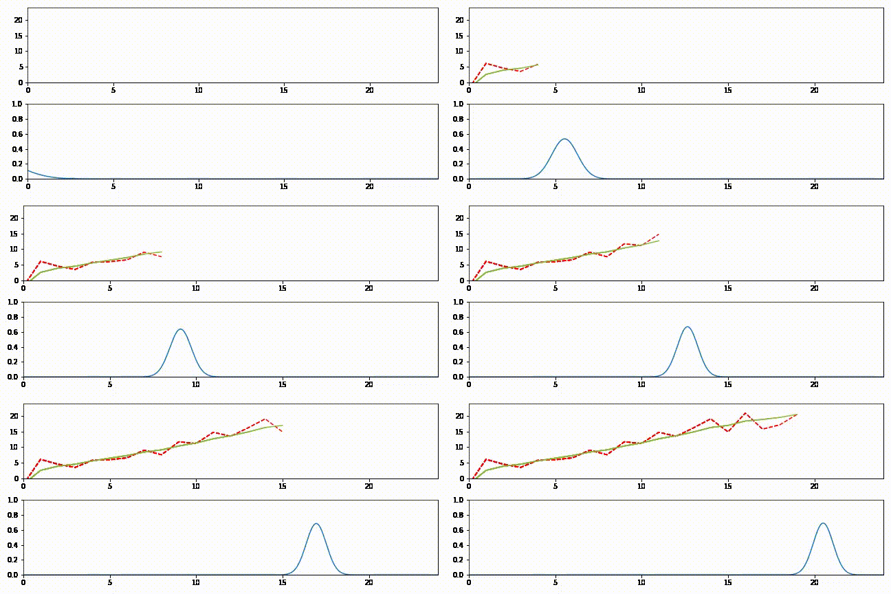
In the example above, the 3 measurements could be combined in 7 ways:
- Only the first measurement is available
- Only the second measurement is available
- Only the third measurement is available
- Only the first and second measurements are available
- Only the first and third measurements are available
- Only the second and third measurements are available
- All three measurements are available
Since combining measurements is done in a loop, simply filling one vector with whichever measurements are available and another vector with their uncertainties will let you combine the available measurements.
resourcescopy link
See my presentation of these concepts at Ctrl^H Hackerspace:
I take a slightly different path to build up to the Kalman filter in the presentation, which might help you see this topic from another perspective.
Additional resources covering Kalman filter design and linear system identification are listed below. Some are sold as published books and others are available for free as digital eBooks.
Kalman and Bayesian Filters in Python includes code samples and eBook. The author simplifies a complex topic for practical application.
Understanding Kalman Filters is a series of videos published by MathWorks. While they look accessible, they skip over a lot of critical context. These tutorials are the principal reason for writing this article.
Special Topics - The Kalman Filter is a series of videos published by Professor Biezen for his online educational site.
Theory of Modal Control published by MIT does a pretty good job of introducing the reader to modeling linear systems.
Estimation II Lecture by Ian Reid at University of Oxford is a quality introduction to Kalman filter design, carefully breaking it down into digestible concepts and keeping math to a minimum.
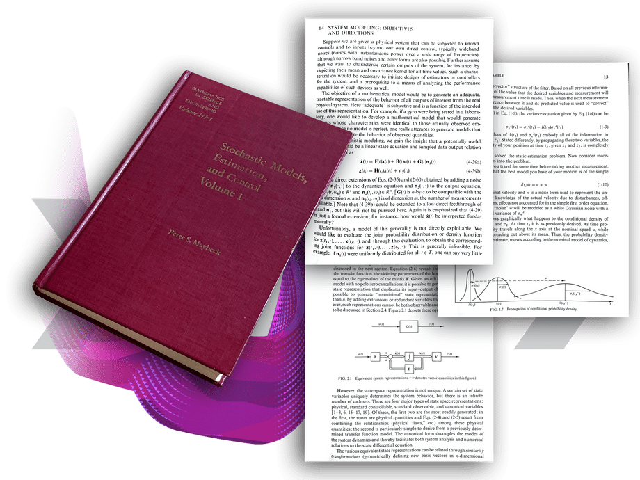
Stochastic Models, Estimation, and Control by Peter Maybeck is approachable and explains where the equations came from:
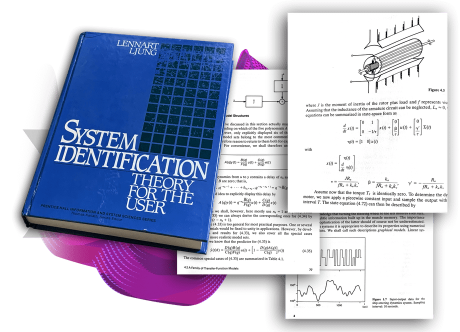
System Identification: Theory for the User by Lennart Ljung requires an undergraduate Mechanical Engineering degree to understand, although a few sections are simple and well-illustrated:
